This post is a supplement to Calculating Returns for Two Kinds of Servicing Fee Schemes.

In the previous post I explored the question of why an investor in Lending Club loans may desire early payment by the borrower, conditional on how servicing fees are levied as well as on the sequence of payments \(\{A_i\}\). I assumed a couple of “simple” instances of \(\{A_i\}\) to make my case, but it’s easy to imagine the more general question of what the best \(\{A_i\}\) an investor could hope for, given \(m\), might be. From an investing standpoint, this isn’t really a useful question to ask—after all, investors don’t get to choose how the borrower repays. But it sounds like it might be an interesting math problem, so why not?

Formally, given \((P_0, r, m, T)\) we’d like to know what sequence of payments \(\{A_i\}_{i=1}^m\) maximizes the investor’s (nominal) IRR, where principal amortizes according to \[ P_i = (1 + r)P_{i-1} - A_i = (1+r)^i P_0 - \sum_{j=1}^i (1+r)^{i-j} A_j. \] In addition, there are constraints \(P_m = 0\) and \(A_i \geq I\) for \(i \neq m\), where \(I\) is the installment \[ I = P_0 \frac{r(1+r)^T}{(1+r)^T - 1}. \]

For the last period, all we need is for the borrower to pay down the remaining principal, i.e., \(A_m = (1 + r)P_{m-1}\), even if \((1+r)P_{m-1} < I\). To make the problem a bit simpler, let’s tack on an explicit constraint \(A_m \geq x\) for some small amount \(x\)—say, $1—instead of allowing \(A_m\) to be arbitrarily small.

With respect to investor fees, let’s consider \(\mathcal{R}_1\) since it’s suggestive of a dynamic tradeoff between fees and interest: on the one hand, the investor would like the principal to amortize quickly to decrease fees, but on the other hand would like it to remain high to earn more interest. The objective, then, is to maximize \(R_1\) satisfying \[ P_0 = \sum_{i=1}^m \left( 1 + \frac{R_1}{12} \right)^{-i} (A_i - s_1 P_i). \]

I already considered two possibilities in the previous post: (1) constant payments \(A_i \equiv A\) and (2) \(m-1\) installments followed by a large \(A_m\). Before trying to find the optimal sequence, let’s take a look at the possibility of (3) a large \(A_1\) followed by the minimum allowable payments in the remaining \(m - 1\) periods. For \(m > 1\) the initial payment can be calculated by first considering a “simpler” sequence of large \(\tilde{A}_1\) followed by \(m - 1\) installments. \(\tilde{A}_1\) needs to be such that \(\tilde{P}_1\) can be paid down in exactly \(m - 1\) installments, i.e., \[ I = \tilde{P}_1 \frac{r(1+r)^{m-1}}{(1+r)^{m-1} - 1}. \] Then (after some algebra) \[ \tilde{P}_1 = P_0 \frac{(1+r)^T - (1+r)^{T-m+1}}{(1+r)^T - 1} \] and \(\tilde{A}_1 = (1+r)P_0 - \tilde{P}_1\). We can then transfer \(I - x\) of payment \(\tilde{A}_m\) to \(\tilde{A}_1\) at rate \(1/(1+r)^{m-1}\), so that \[ A_1 = \tilde{A}_1 + \frac{I - x}{(1+r)^{m-1}}. \] (If this isn’t apparent, read on for an explanation.)

We can reuse the functions from the previous post, modifying gen_A_seq accordingly:

A = function(P0, r, m) {
  # P0 -- initial principal
  # r  -- interest rate (monthly)
  # m  -- number of payment periods
  P0 * r * (1 + r)^m / ((1 + r)^m - 1)
}

P_i = Vectorize(
  # Compute outstanding principal after i payments
  function(A_seq, P0, r, i) {
    # A_seq -- sequence of payments (length m)
    if (i==0) return(P0)
    (1 + r)^i * P0 - sum(A_seq[1:i] * (1 + r)^((i-1):0))
  },
  vectorize.args = 'i')

gen_A_seq = function(P0, r, m, Term=36, k) {
  # k -- switch number
  switch(
    k, {
      # 1 -- Constant payments
      rep(A(P0, r, m), m)
    }, {
      # 2 -- m - 1 installments followed by large A_m
      Inst = A(P0, r, Term)
      A_seq = rep(Inst, m - 1)
      c(A_seq, (1 + r) * P_i(A_seq, P0, r, m - 1))
    }, {
      # 3 -- Large A_1, if (m > 1) m - 2 installments, A_m = 1
      if (m==1) return((1 + r) * P0)
      Inst = A(P0, r, Term)
      P1  = P0 * ((1 + r)^Term - (1 + r)^(Term - m + 1)) / ((1 + r)^Term - 1)
      A1 = (1 + r)*P0 - P1 + (Inst - 1) / (1 + r)^(m-1)
      c(A1, rep(Inst, m - 2), 1)
    }
  )
}

R1 = Vectorize(
  function(s, P0, r, m, k) {
    # s -- service fee rate (monthly, on remaining principal)
    # P0, r, m -- args to A()
    # k -- switch number (payment sequence 1, 2, or 3)
    A_seq = gen_A_seq(P0, r, m, k=k)
    fun = function(z) (P0 - sum((1 + z/12)^-(1:m) *
                                  (A_seq - s * P_i(A_seq, P0, r, 1:m))))^2
    # solve for IRR
    optimize(fun, interval=c(0, .5))$minimum
  },
  vectorize.args = 'm')

Also keeping with the previous post, let’s make the test case a loan with $1000 principal and 15% annual interest rate, with service fee rate \(s_1\) equal to 1.3% per annum.

# Compute the IRR for each m, for each sequence -- 36 x 3 matrix
IRR = sapply(1:3, function(k) R1(s=.013/12, P0=1000, r=.15/12, m=1:36, k))

matplot(1:36, IRR, las=1, type='l',
        xlab='Months until full payment (m)',
        ylab='Internal rate of return')
legend('topright', c('(1) Constant A', '(2) Large A_m', '(3) Large A_1'),
       lty=1:3, col=c('black','red','green'), inset=.01)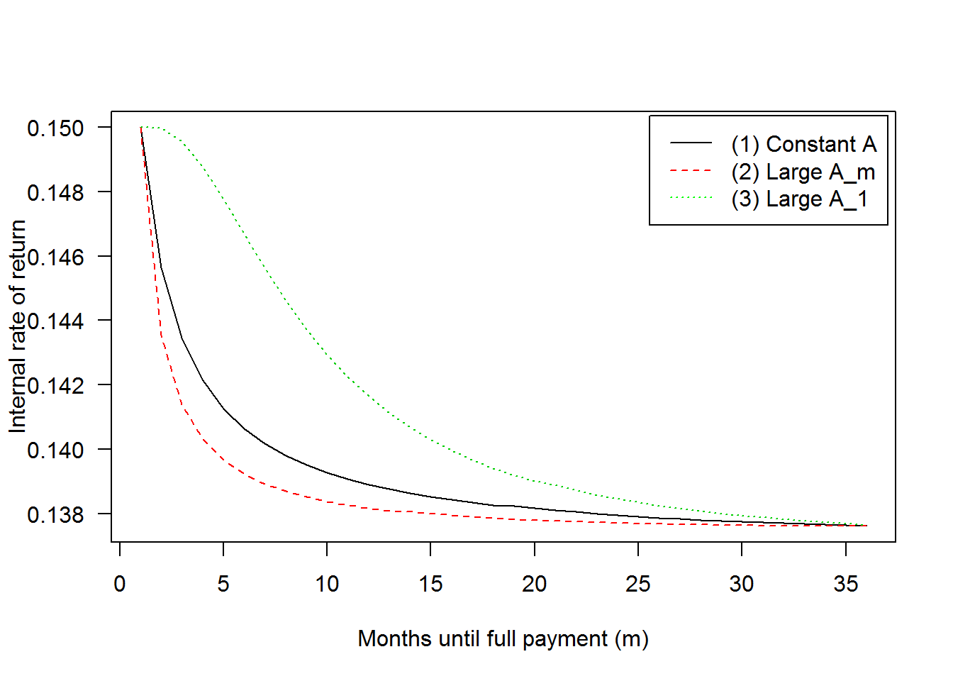

Sequence (3) is rather extreme in that payment is front-loaded as much as possible without violating any of the constraints. As it turns out, it is also optimal. To prove it, I’ll use (3) as a starting point and show that moving part of payment \(A_1\) downstream to \(A_j\) (the only permissible action since only \(A_1\) is not already bound by a constraint) cannot increase \(R_1\). Since any permissible \(\{A_i\}\) (given \(m\)) can be constructed starting from (3) and redistributing payment from \(A_1\), it will follow that (3) must be the optimal sequence.

Let me first introduce the notation \(dX/dA_{i \rightarrow j}\) to describe the marginal change in \(X\) from transferring a marginal amount of \(A_i\) to \(A_j\), holding all other payments fixed, and in such a way that the constraint \(P_m = 0\) remains satisfied. (More conventionally, this can be thought of as a directional derivative \(\nabla_\textbf{v} X\), where \(\textbf{v}\) is an \(m\)-dimensional unit vector with non-zero components \(v_i\) and \(v_j\).¹) The claim, then, is that \(dR_1/dA_{1 \rightarrow j} \leq 0\) for all \(1 < j \leq m\).

Importantly, \(A_{i \rightarrow j}\) cannot be 1:1 due to compounding. In particular, while \(dA_i/dA_{i \rightarrow j} = -1\), \[ \frac{dA_j}{dA_{i \rightarrow j}} = (1+r) \frac{dP_{j-1}}{dA_i} = (1 + r)^{j-i}. \] This ensures that \(P_j\) remains unchanged, and therefore that the remaining payments \(\{A_i\}_{i > j}\) still lead to \(P_m = 0\). (To avoid ambiguity, define \(dA_j/dA_{i \rightarrow j} = 0\) when \(j=i\).)²

Calculating \(dR_1/dA_{1 \rightarrow j}\) is a little bit tricky because \(R_1\) is defined implicitly in the objective function; we’ll need to use implicit differentiation. Taking derivatives of both sides of the objective function (defining \(\beta = (1 + R_1/12)^{-1}\) to simplify notation) and rearranging yields \[ \frac{dR_1}{dA_{1 \rightarrow j}} = \frac{ -\beta + \beta^j (1+r)^{j-1} - s_1 \sum_{i=1}^{j-1} \beta^i (1+r)^{i-1}}{ \frac{1}{12}\sum_{i=1}^m i \beta^{i+1} (A_i - s_1 P_i) } \] (See here for a step-by-step derivation.) Assuming that \(s_1\) is not too large so that the denominator is positive, \(dR_1/dA_{1 \rightarrow j} \leq 0\) when the numerator is non-positive, i.e., when \[ z^{j-1} - s_1 \frac{1 - z^{j-1}}{1 - z} \leq 1, \] where \(z = \beta(1+r)\). Since \(R_1\) cannot be higher than the interest rate, \(z \geq 1\), and the above inequality can be rearranged to \(s_1 \geq 1 - z\), which always holds as \(s_1\) is assumed to be non-negative. Thus, \(dR_1/dA_{1 \rightarrow j} \leq 0\) unconditionally for all \(j\), with strict inequality if \(s_1 > 0\).