This post is a supplement to A Note on Lending Club and Institutional Investment, which shows that institutional investors tend to fund loans that will be prepaid. Below is a short mathematical justification for why it makes sense for them to do so, given Lending Club’s policy on servicing fees. I also include retail investors for comparison.

Suppose we’d like to compute the internal rate of return¹ (IRR) for a loan investment based on two different fee schemes. The first (call it \(\mathcal{R}_1\)) charges a fee \(s_1\) in proportion to each period’s outstanding principal balance, while the second (\(\mathcal{R}_2\)) charges a fee \(s_2\) on all payments by the borrower, up to the contractual monthly payment in the first 12 months.² (\(\mathcal{R}_1\) and \(\mathcal{R}_2\) represent fees levied on institutional (whole loan) investors and retail (Note) investors, respectively.) The borrower can “prepay” a loan with term \(T\) by paying off the entire principal in \(m < T\) months. Given initial principal \(P_0\), monthly interest rate \(r\), payment periods \(m\), and payment sequence \(\{A_i\}_{i=1}^m\), the principal amortizes according to \[ P_i = (1+r)P_{i-1} - A_i = (1+r)^i P_0 - \sum_{j=1}^i (1+r)^{i-j} A_j \] and the corresponding IRRs \(R_1\) and \(R_2\) satisfy \[ P_0 = \sum_{i=1}^m \left(1 + \frac{R_1}{12} \right)^{-i} (A_i - s_1 P_i) \\ P_0 = \sum_{i=1}^m \left(1 + \frac{R_2}{12} \right)^{-i} \big(A_i - s_2 Y_i \big), \] where \(Y_i = \min(I, A_i)\) if \(i \leq 12\) and \(A_i\) otherwise, and \(I\) is the installment (or minimum payment) given by \[ I = P_0 \frac{r(1+r)^T}{(1+r)^T - 1}. \]

Note that in the amortization formula, \(P_i\) represents the principal at the “end” of period \(i\), i.e., after payment \(A_i\) is made. I deliberately modeled it this way since \(\mathcal{R}_1\) fees are calculated on end-of-month principal, per Lending Club policy.³ I also assume that payments are large enough to at least cover interest, i.e., \(A_i \geq rP_{i-1}\), as the principal can never increase.

Now all that remains is to specify \(\{A_i\}\). First assuming constant monthly payments given \(m\), \[ A_i = P_0 \frac{r(1+r)^m}{(1+r)^m - 1} \equiv A, \] we can use the following code to see how \(R_1\) and \(R_2\) vary with \(m\). Note that by construction, i.e., by the choice of \(\{A_i\}\), we have \(P_m = 0\). Also note that the result doesn’t depend on \(P_0\), though I’ve kept it to make the calculations more explicit.

A = function(P0, r, m) {
  # P0 -- initial principal
  # r  -- interest rate (monthly)
  # m  -- number of payment periods
  P0 * r * (1 + r)^m / ((1 + r)^m - 1)
}

P_i = Vectorize(
  # Compute outstanding principal after i payments
  function(A, P0, r, i) {
    if (i==0) return(P0)
    (1 + r)^i * P0 - A * sum((1 + r)^((i-1):0))
  },
  vectorize.args = 'i')

R1 = Vectorize(
  function(s, P0, r, m) {
    # s -- service fee rate (monthly, on remaining principal)
    # P0, r, m -- args to A()
    A_ = A(P0, r, m)
    fun = function(z) (P0 - sum((1 + z/12)^-(1:m) *
                                  (A_ - s * P_i(A_, P0, r, 1:m))))^2
    # solve for IRR
    optimize(fun, interval=c(0, .5))$minimum
  },
  vectorize.args = 'm')

R2 = Vectorize(
  function(s, P0, r, m) {
    # s  -- service fee rate (monthly, on payments)
    # P0, r, m -- args to A()
    A_ = rep(A(P0, r, m), m)
    Y_ = replace(A_, 1:min(m, 12), A(P0, r, 36))
    fun = function(z) (P0 - sum((1 + z/12)^-(1:m) *
                                  (A_ - s * Y_)))^2
    # solve for IRR
    optimize(fun, interval=c(0, .5))$minimum
  },
  vectorize.args = 'm')

The test case below is a loan with $1000 principal and 15% annual interest rate, with fees \(s_1\) and \(s_2\) equal to 1.3% per annum and 1%, respectively. (According to Lending Club’s policy for whole loans, \(s_1\) is variable but 1.3% per annum is the highest servicing fee it will charge. A lower \(s_1\) will increase \(R_1\), up to the interest rate when \(s_1 = 0\).)

# Returns for institutional (whole loan) investors
r_inst = R1(s=.013/12, P0=1000, r=.15/12, m=1:36)

# Returns for retail (Note) investors
r_ret  = R2(s=.01, P0=1000, r=.15/12, m=1:36)

matplot(1:36, cbind(r_inst, r_ret), las=1, type='l',
        xlab='Months until full payment (m)',
        ylab='Internal rate of return')
legend('topright', c('R1','R2'), lty=c(1,2), col=c('black','red'),
       inset=.01)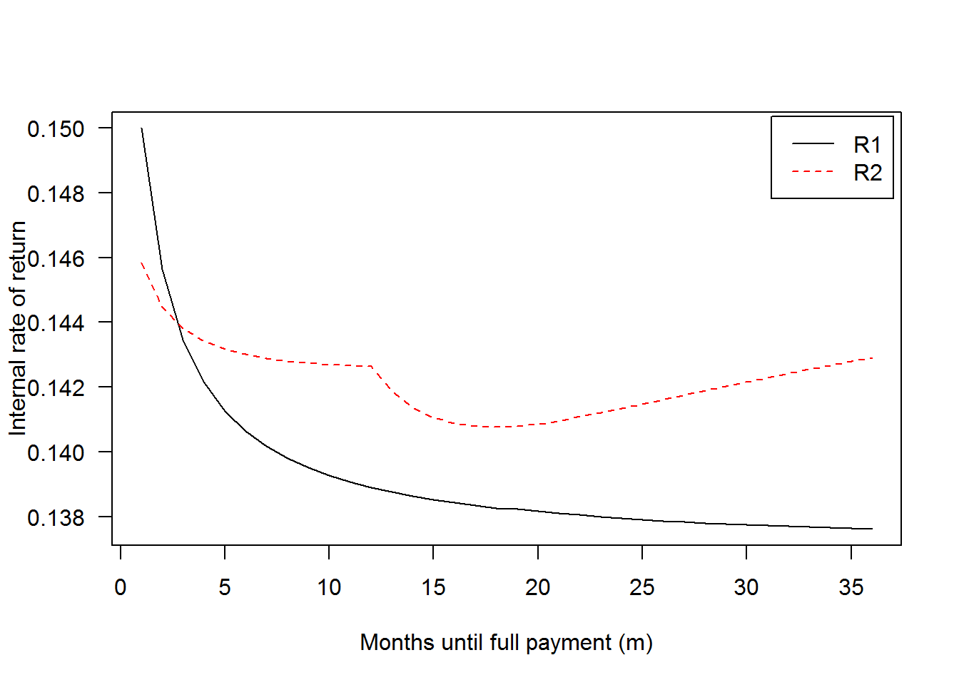

This isn’t a complete picture since it doesn’t account for returns from reinvestment (purchasing new Notes or whole loans after receiving each \(A_i\), which can be done recursively). But it’s clear that investors who are charged fees under scheme \(\mathcal{R}_1\) can achieve a higher return with early payment, i.e., $ \Delta_m R_1 < 0$. The gains are relatively small but may be significant for investors with very large portfolios. With prepayment protection, early payment is also the most desirable outcome under scheme \(\mathcal{R}_2\), although the curve is upward-sloping for \(m > 17\).

We can’t yet declare the matter settled as there’s a potential problem with the above graph. Empirically, given \(m\), the borrower tends to back-load prepayment to later periods, so the assumption of fixed payments isn’t very realistic. (I checked this using Lending Club’s payments data, but I’ll defer the evidence to a future post.) A more realistic flow of payments would be constant installments for \(m-1\) periods and one large payment to expunge all outstanding principal (with interest) in period \(m\).

It’s straightforward to modify the functions above to accomodate non-constant payments:

P_i = Vectorize(
  # Compute outstanding principal after i payments
  function(A_seq, P0, r, i) {
    # A_seq -- sequence of payments (length m)
    if (i==0) return(P0)
    (1 + r)^i * P0 - sum(A_seq[1:i] * (1 + r)^((i-1):0))
  },
  vectorize.args = 'i')

gen_A_seq = function(P0, r, m, Term=36) {
  # Sequence of m - 1 installments, plus final payment (1+r)*P_{m-1}
  Inst = A(P0, r, Term)
  A_seq = rep(Inst, m - 1)
  c(A_seq, (1 + r) * P_i(A_seq, P0, r, m - 1))
}

R1 = Vectorize(
  function(s, P0, r, m) {
    # s -- service fee rate (monthly, on remaining principal)
    # P0, r, m -- args to A()
    A_seq = gen_A_seq(P0, r, m)
    fun = function(z) (P0 - sum((1 + z/12)^-(1:m) *
                                  (A_seq - s * P_i(A_seq, P0, r, 1:m))))^2
    # solve for IRR
    optimize(fun, interval=c(0, .5))$minimum
  },
  vectorize.args = 'm')

R2 = Vectorize(
  function(s, P0, r, m=36) {
    # s  -- service fee rate (monthly, on payments)
    # P0, r, m -- args to A()
    A_seq = gen_A_seq(P0, r, m)
    Y_seq = replace(A_seq, 1:min(m, 12), A(P0, r, 36))
    fun = function(z) (P0 - sum((1 + z/12)^-(1:m) *
                                  (A_seq - s * Y_seq)))^2
    # solve for IRR
    optimize(fun, interval=c(0, .5))$minimum
  },
  vectorize.args = 'm')

# Returns for institutional (whole loan) investors
r_inst = R1(s=.013/12, P0=1000, r=.15/12, m=1:36)

# Returns for retail (Note) investors
r_ret  = R2(s=.01, P0=1000, r=.15/12, m=1:36)

matplot(1:36, cbind(r_inst, r_ret), las=1, type='l',
        xlab='Months until full payment (m)',
        ylab='Internal rate of return')
legend('topright', c('R1','R2'), lty=c(1,2), col=c('black','red'),
       inset=.01)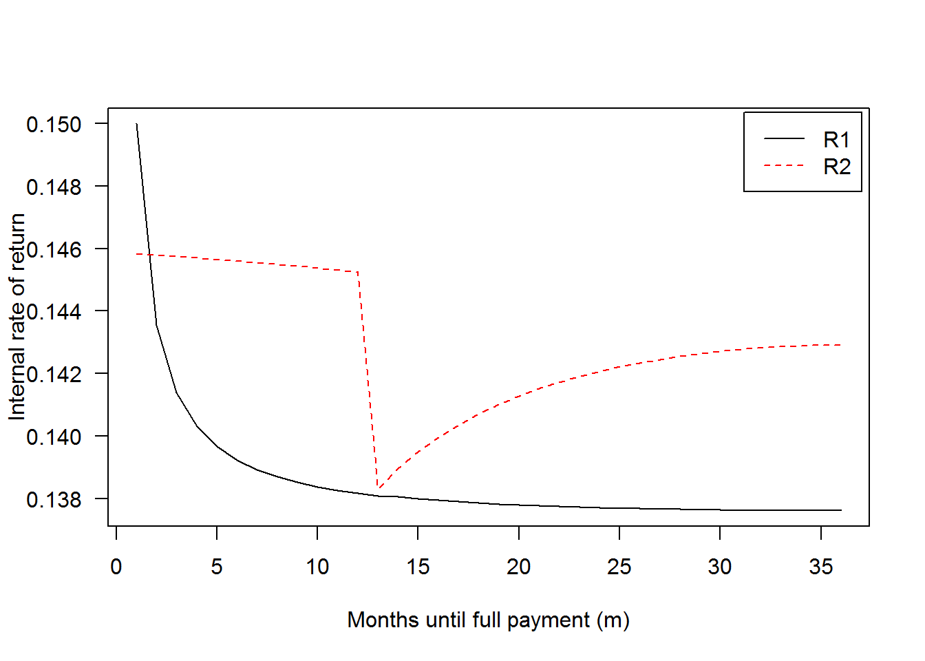

With this more realistic payment sequence, an investor will still desire early payment under \(\mathcal{R}_1\), although he will face strictly lower returns for all \(m \notin \{1, 36\}\). In particular, the slope of the curve \(R_1(m)\) is even more severe for small \(m\), corresponding to a larger “penalty” on returns of one additional month. In contrast, returns are higher under \(\mathcal{R}_2\) for \(m \leq 12\), although \(m > 12\) yields lower returns since prepayment protection will not extend to the large final payment. Note that the endpoints of the two curves are the same as before since the two versions of \(\{A_i\}\) are identical for \(m = 1\) and \(m = T\).

To give a better sense of the role of prepayment protection, I’ll add a line for a scheme (call it \(\mathcal{R}_2^a\)) which charges a 1% fee on all borrower payments. The difference is stark:

R2a = Vectorize(
  function(s, P0, r, m=36) {
    # s  -- service fee rate (monthly, on payments)
    # P0, r, m -- args to A()
    A_seq = gen_A_seq(P0, r, m)
    fun = function(z) (P0 - sum((1 + z/12)^-(1:m) *
                                  (1 - s) * A_seq))^2
    # solve for IRR
    optimize(fun, interval=c(0, .5))$minimum
  },
  vectorize.args = 'm')

# Returns for retail (Note) investors, no prepayment protection
r_ret_no_protection = R2a(s=.01, P0=1000, r=.15/12, m=1:36)

matplot(1:36, cbind(r_inst, r_ret, r_ret_no_protection), las=1, type='l',
        col=c('black','red','darkred'),
        xlab='Months until full payment (m)',
        ylab='Internal rate of return')
legend('bottomright', c('R1','R2','R2a'), lty=1:3, col=c('black','red','darkred'),
       inset=.01)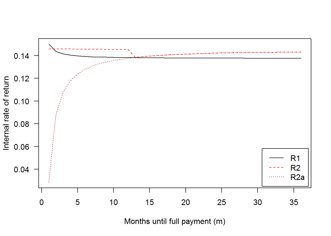

Keep in mind that these examples only evaluate ex-post returns; when an investor is actually choosing loans on Lending Club, \(m\) and \(\{A_i\}\) are unknown and there is non-negligible risk of borrower default. If prepayment and default are both correlated with variable \(X\), then selecting on \(X\) may diminish gains from prepayment compared to above.