R comes with a number of built-in functional programming tools, one of which is the Reduce function which recursively calls a binary function over a vector of inputs. It’s quite versatile, but most explanations of Reduce tend to focus on trivial use cases that are not particularly inspiring. Even Hadley Wickham’s Advanced R—which I highly recommend as a reference—limits the discussion to implementations of cumulative sum—for which there is already cumsum—and multiple intersect. I’ll use this post to demonstrate some less obvious examples of how Reduce can come in handy, based on an alternative interpretation of the function as a simple kind of state machine. The examples aren’t necessarily applicable to day-to-day data analysis tasks, but should be interesting enough to impart a more expansive understanding of what Reduce can do.

If you’ve never heard of Reduce or have never thought to use it before, I recommend taking a quick look at this or this or this before reading further.

I think it’s appropriate to start by revisiting an example from Advanced R where Hadley claims it is not possible to use a functional. Of a for-loop implementation of an exponential moving average (also exponential smooth), he writes, “We can’t eliminate the for-loop because none of the functionals we’ve seen allow the output at position i to depend on both the input and output at position i-1” (Chapter 11, page 226).

This is precisely what Reduce does! In fact, given x and smoothing parameter alpha, we can compute the EMA without using an explicit for-loop¹:

exps <- function(x, alpha) {
  Reduce(function(s, x_) alpha*x_ + (1-alpha)*s, x, accumulate=TRUE)
}

x <- cumsum(rnorm(100))

plot(x, type='l')
lines(exps(x, alpha=.2), col='red')
lines(exps(x, alpha=.4), col='blue')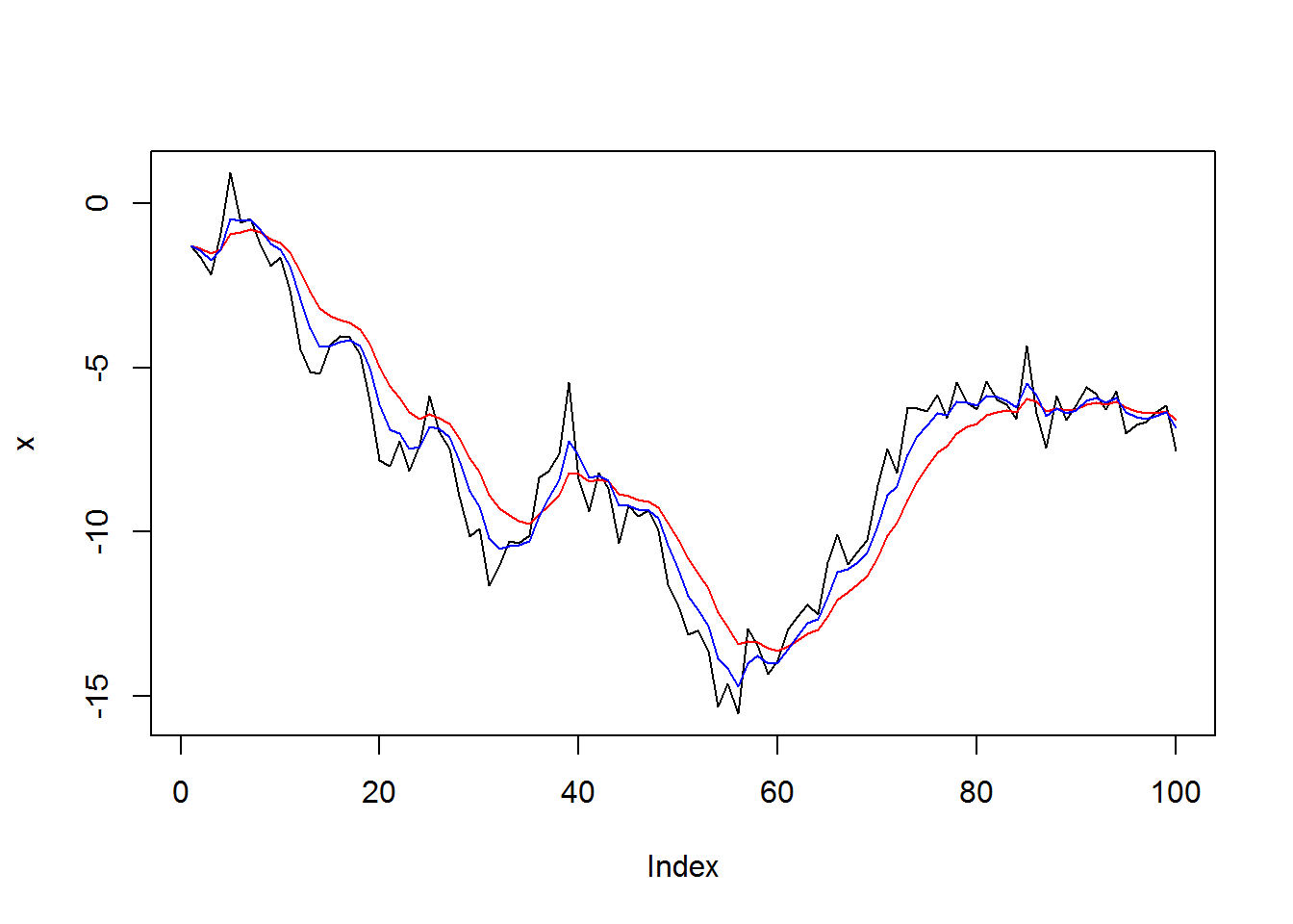

(As a reminder, specifying accumulate=TRUE causes Reduce to return all intermediate results, so that the output has the same length as x. We can also specify an initial value with the init argument, in which case the output will have length length(x) + 1.)

More generally, Reduce can implement a state machine where the state is updated according to its previous value and an input (or an “action”), i.e., $ s' = f(s, a) $.² In the EMA example, the state is s and the input is x_, an element of x. This conception of Reduce is related to the idea of applying a binary function recursively, but perhaps provides a more natural way of thinking about certain kinds of problems.

To see this in a second example, suppose that we’d like to compute a cumulative sum that “resets” after encountering the value zero. All we need to do is write a function that takes the current sum (the state) as given, and either adds to or resets that sum depending on the value of the input:

x <- c(1, 2, 4, 0, -1, 3, 0, 1, 1, 1)

Reduce(function(s, x_) (s + x_)*(x_ != 0), x, accumulate=TRUE)
##  [1]  1  3  7  0 -1  2  0  1  2  3

Since we didn’t specify init as an argument, the first value of x serves the role of the initial state. To get the “next” value of the state, Reduce computes $ f(1, 2) = (1 + 2)*(2 \neq 0) = 3 $, then $ f(3, 4) = (3 + 4)*(4 \neq 0) = 7 $ and so on, producing the printed output.

How about a cumulative mean? We can use the formula for an online update of the mean, which is useful for large data when observations are encountered sequentially: \[ \bar{x}_{n+1} = \frac{n}{n+1} \bar{x}_n + \frac{1}{n+1} x_{n+1}. \] Note that Reduce will need to be able to access and update the value \(n\), which can be accomplished by wrapping the computation in a function and using the upstream assignment operator <<-:

cummean <- function(x) {
  n <- 0
  Reduce(function(s, x_) {
    n <<- n + 1
    n/(n + 1) * s + x_/(n + 1)
  }, x, accumulate=TRUE)
}

(x <- round(rnorm(15), 2))
##  [1]  0.51 -1.16  0.67 -0.55 -0.34  0.12 -0.79  0.49  0.24  0.12 -0.12  0.18
## [13] -0.66 -1.89  1.35
round(cummean(x), 2)
##  [1]  0.51 -0.32  0.01 -0.13 -0.17 -0.12 -0.22 -0.13 -0.09 -0.07 -0.07 -0.05
## [13] -0.10 -0.23 -0.12

We can also use Reduce to implement a version of zoo::na.locf (“last observation carry forward”), which replaces NA with the last non-NA value:

x <- rep(NA_integer_, 14)
x[sample(length(x), 5)] <- 1:5
x
##  [1]  1 NA NA  3 NA NA NA NA NA  4  5  2 NA NA

Reduce(function(s, x_) if (is.na(x_)) s else x_, x, accumulate=TRUE)
##  [1] 1 1 1 3 3 3 3 3 3 4 5 2 2 2

The function simply returns s if the input x_ is NA; otherwise x_ becomes the new s.

Now suppose we have a vector of 0, 1, and -1 which represent actions peformed on some state which can be 0 or 1. If the action “1” is performed, the state switches to (or remains) “1”; if “0” is performed, there is no effect; and if “-1” is performed, the state switches to (or remains) “0”. (Think of this as flipping a light switch on or off.) We can use Reduce to compute the values of the state given a sequence of actions A and an initial state:

(A <- sample(c(-1,0,1), size=14, replace=TRUE))
##  [1]  0  1  1  0  0 -1  0  1  1  1  0  0  0  0

Reduce(function(s, a_) as.integer(s + a_ > 0), A, init=1L, accumulate=TRUE)
##  [1] 1 1 1 1 1 1 0 0 1 1 1 1 1 1 1

I’ve used this as a method to strip away blocks³ of unnecessary text (headers, footers, etc.) from multi-page PDFs after text conversion. All I need to do is mark the rows where the useful data and the useless text begin, then Reduce and drop.

All of the examples so far have used scalar (really, atomic vectors of length 1) states and inputs, but it’s straightforward to work with more complex object types like matrices and data frames. We could use Reduce to merge a list of data frames (a common data analysis task), or to simulate sample paths for a multivariate time series where the state is a vector $S$.

There’s even a way to make Reduce handle multiple input arguments. Say we want to recursively compute $ s' = a_1 \times s + a_2 $ given a sequence of $ (a_1, a_2) $ pairs. We can use Map (another useful functional) to combine A1 and A2 pairwise and then use standard indexing to access the different inputs:

A1 <- rnorm(10)
A2 <- rnorm(10)

Reduce(function(s, a) a[1] * s + a[2], Map(c, A1, A2), init=1L, accumulate=TRUE)
##  [1]  1.00000000 -0.88894348 -0.18750589 -0.72132054 -1.88857905 -0.11068876
##  [7] -0.07506955 -0.81876347  0.67835055 -0.29723727 -1.56577053

# or:
# Reduce(function(s, a) rnorm(1) * s + rnorm(1), seq_len(10), init=1L, accumulate=TRUE)

One last example from StackOverflow. Say we have a binary vector x and want to replace the two elements following every “1” with “1”. We can use Reduce to create a counter that decrements by 1 in the case of “0” and resets to 3 in the case of “1”, so that any two “0” elements following a “1” correspond to positive values in the counter. Taking the sign then gives the desired result:

x <- rep(0, 14)
x[sample(length(x), 5)] <- 1
x
##  [1] 0 0 1 0 0 0 0 1 0 1 1 0 0 1

(counter <- Reduce(function(s, x_) min(3, max(s-1, 0) + x_), 3*x, accumulate=TRUE))
##  [1] 0 0 3 2 1 0 0 3 2 3 3 2 1 3

sign(counter)
##  [1] 0 0 1 1 1 0 0 1 1 1 1 1 1 1

This solution takes some thought, and perhaps an alternative method would be preferable for the sake of readability. But the point is that Reduce is flexible enough to be a contender for a much wider range of problems than is usually recognized. My hope is that the above examples help illuminate how Reduce (and functional programming) can be used cleverly to provide compact solutions for certain kinds of programming problems.