The Data

The downloadable files are large—almost 6 GB each—but contain redundancies, as constant loan attributes are recorded for every (loan, payment) row. These “fixed” attributes can be spliced off and saved to a separate file, reducing the total file size to under 4 GB—small enough to fit in memory.³

library(data.table) # using v1.10.5 (dev)
library(ggplot2)

ph_fixed = fread('paymentHistory_fixed.csv', key='loan_id')
ph_master = fread('paymentHistory.csv', key=c('loan_id','mob'))

As the file names suggest, paymentHistory_fixed.csv contains the fixed attributes for each loan id, and paymentHistory.csv contains the breakdown of borrowers’ month-by-month payments. The following variables are available:

In ph_fixed:

• loan_id – Unique loan identifier.

• interestrate – The interest rate.

• term – The term, either 36 months or 60 months.

• grade – Letter grade in A–G assigned to the loan based on “the credit quality and underlying risk of the borrower.”

• vintage – The year-quarter of issuance.

• Other variables: monthlycontractamt, dti, state, appl_fico_band, homeownership, …

In ph_master:

• loan_id – Unique loan identifier.

• mob – Number of months after loan issuance (index for the payment period).

• pbal_beg_period – Remaining principal balance at the beginning of the payment period.

• due_amt – The amount due.

• Breakdown of the payment received (identical set of variables with suffix _inv corresponds to payment received by investors; different if loan received partial funding from Lending Club):

  • prncp_paid – Amount of principal paid.

  • int_paid – Amount of interest paid.

  • fee_paid – Amount of late fees paid.

  • coamt – Charge-off amount.

  • pco_recovery – Amount recovered in case of charge-off.

  • pco_collection_fee – Amount of recovery collection fees in case of charge-off.

• received_d – Date the period’s payment was received.

• period_end_lstat – The loan status at the end of the payment period. One of {“Issued”, “Current”, “In Grace Period”, “Late (16-30 days)”, “Late (31-120 days)”, “Default”, “Charged Off”, “Fully Paid”}.

The variable initial_list_status is available in the public data and identifies whether a loan was initially listed in the whole (W) or fractional (F) market. Loans listed “whole” become available for fractional funding (and vice versa) if there are no buyers within a certain time frame. To determine whether a loan was actually funded by a whole loan investor, we use this in conjunction with num_investors which is scraped from individual “loan detail” pages (example screencap below).⁴ The uptake of whole loans varies significantly over time and across loan grades but is typically 70-80 percent overall.

Sample “loanDetail.action” page which includes field showing number of investors

The following code chunk merges in these additional variables and transforms the data:

additional = fread('additional.csv')
setnames(additional, 'initial_list_status', 'ils')
ph_fixed = additional[ph_fixed, on='loan_id']
rm(additional)

# Month of issuance
ph_fixed[, `:=`(issueMon = zoo::as.yearmon(issueddate, '%b%Y'), issueddate = NULL)]

# Number of payment periods elapsed since issuance
ph_fixed[, numPay:= 12*(zoo::as.yearmon('Aug 2017') - issueMon)]

# Correct discrepancies in num_investors (Found evidence that whole loans
# no longer pushed into fractional market after buffer period, starting
# Jun 2016. So every W loan must have 1 investor.)
ph_fixed[ils=='W' & issueMon >= 'Jun 2016', num_investors:= 1]

# Pool grades F and G (small sample size)
ph_fixed[grade %in% c('F','G'), grade:= 'FG']

# Identify investor types using initial_list_status & num_investors
ph_fixed[ils=='W' & num_investors==1, investor_type:= 'W']
ph_fixed[ils=='F' | num_investors>=2, investor_type:= 'F']

# Compute the fraction of funding via notes using sales reports data
ph_fixed[is.na(funded_amt_lc), funded_amt_lc:= 0]
ph_fixed[, funded_amt_inv:= funded_amt - funded_amt_lc]
ph_fixed[, note_wgt:= ifelse(is.na(sold_amt), 0, (sold_amt-funded_amt_lc)/funded_amt_inv)]

Analysis

One important dimension along which aggregate portfolios might differ is the time to full repayment by borrowers, who must pay the installment at minimum but can prepay if desired. With prepayment, a loan may be fully paid well before the maturity date, and consequently investors will lose future interest payments.

Apropos of this idea, the following code chunk computes the fraction of loans, by grade and investor type, which reached a terminal state—either “fully paid” (fp) or “charged off” (co)—by month \(i\), for \(1 \leq i \leq T\). I restrict the sample to 3-year loans, so \(T = 36\). (There are also 5-year loans which I ignore for simplicity.) The filter numPay >= i ensures that only borrowers who could have possibly made \(i\) payments are counted in the denominator (i.e., excluding loans that were issued fewer than \(i\) months ago).

bigT = 36
w_id = ph_fixed[investor_type=='W' & term==bigT & issueMon >= 'Sep 2012',
                .(loan_id, numPay, grade)]
f_id = ph_fixed[investor_type=='F' & term==bigT & issueMon >= 'Sep 2012',
                .(loan_id, numPay, grade)]

# By grade g and months after issuance mob:
# w_fp, f_fp -- number of whole (fractional) loans fully paid
# w_co, f_co -- number of whole (fractional) loans charged off
terminal = CJ(grade=ph_fixed$grade, mob=1:bigT, unique=TRUE)
terminal[, c('w_fp','f_fp','w_co','f_co','nw','nf'):= NA_real_]

for (g in terminal[, unique(grade)]) {
  cat('Grade', g, '\n')
  
  for (i in 1:bigT) {
    cat(i); if (i<bigT) cat(',') else cat('\n')
    w_ids = w_id[numPay >=i & grade==g, loan_id]
    f_ids = f_id[numPay >=i & grade==g, loan_id]
    
    terminal[J(g,i), `:=`(
      w_fp = ph_master[J(w_ids)][mob <= i,
                                 sum(period_end_lstat=='Fully Paid')],
      f_fp = ph_master[J(f_ids)][mob <= i,
                                 sum(period_end_lstat=='Fully Paid')],
      w_co = ph_master[J(w_ids)][mob <= i,
                                 sum(period_end_lstat=='Charged Off')],
      f_co = ph_master[J(f_ids)][mob <= i,
                                 sum(period_end_lstat=='Charged Off')],
      nw = length(w_ids),
      nf = length(f_ids))]
    
  }; rm(i, w_ids, f_ids)
  
}; rm(g)

# Compute fractions from counts
terminal[, `:=`(
  w_fp = w_fp/nw, f_fp = f_fp/nf, w_co = w_co/nw, f_co = f_co/nf,
  all_fp = (w_fp + f_fp)/(nw + nf), all_co = (w_co + f_co)/(nw + nf))]

# Reshape wide --> long
terminal.long = melt(terminal, id=key(terminal), patterns('_fp','_co'),
                     value.name=c('Fully paid', 'Charged off'))

levels(terminal.long$variable) <- c('Whole','Fractional','All')
setkey(terminal.long, variable, grade, mob)

The plots below reveal two interesting empirical facts about aggregate portfolios. First, loans funded by institutional investors are paid off sooner than those funded by retail investors, even though the overall default rates (measured from the top) are slightly higher. This holds true within all loan grades, so it cannot be the result of differing selection with respect to grade.

ggplot(terminal.long[!'All'], aes(x=mob, y=100*`Fully paid`, color=variable)) +
  geom_line() +
  geom_point(data=function(d) d[mob==bigT]) +
  geom_line(aes(y=100*(1-`Charged off`)), lty='dashed') +
  geom_point(data=function(d) d[mob==bigT], aes(y=100*(1-`Charged off`))) +
  scale_color_manual('', values=c(Fractional='blue', Whole='red')) +
  scale_x_continuous(breaks=seq(0,bigT,6)) +
  scale_y_continuous(breaks=seq(0,100,20)) +
  facet_wrap('grade', ncol=2) +
  labs(x='Months since issuance', y='',
       title='Time to Terminal Status, 3-Year Loans, by Grade',
       subtitle='Percent fully paid (solid) or charged off (dashed)') +
  theme(legend.pos='top')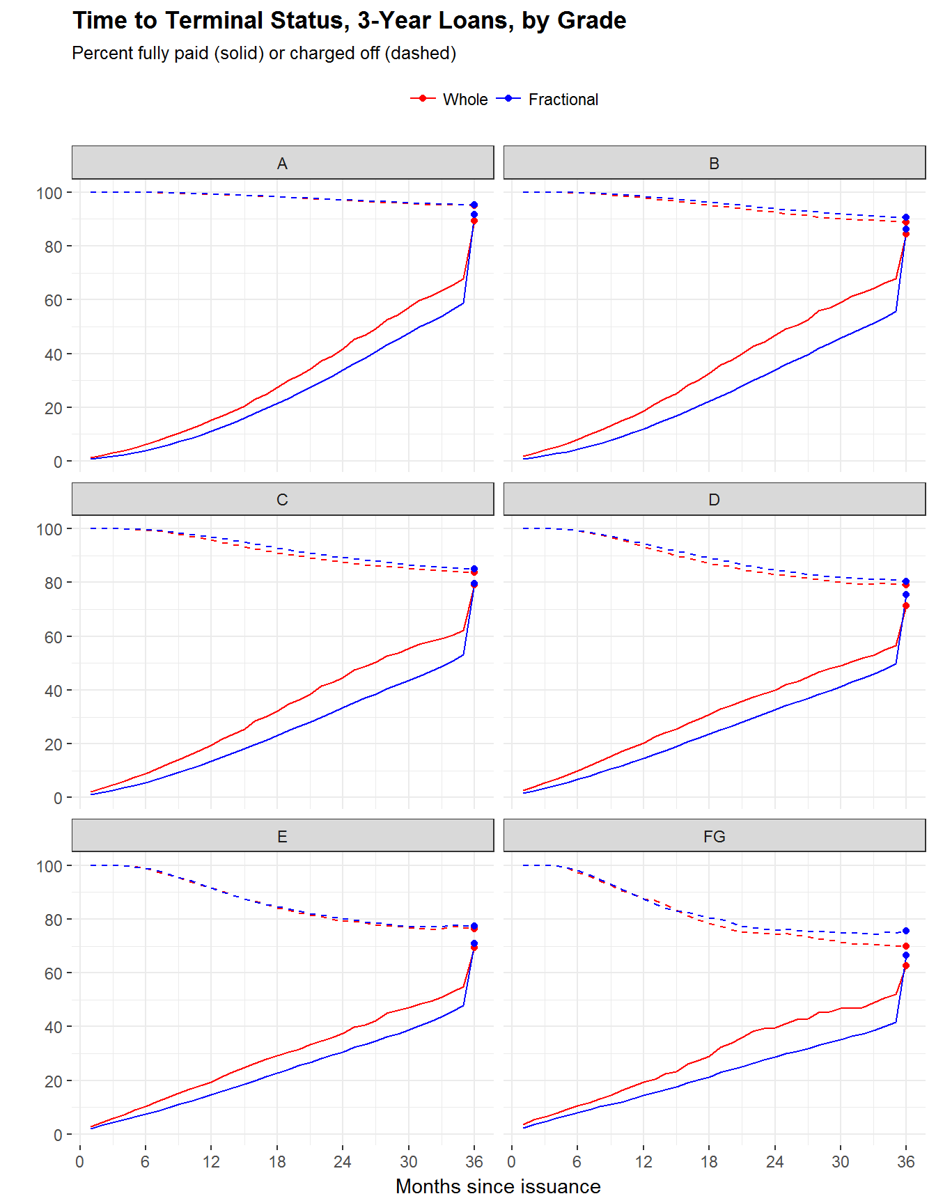

The next code chunk below computes the fraction of whole loan offerings funded by institutional investors (“uptake”), conditional on vintage and the ex-post realization of months until full repayment. The top of the corresponding plot is dominated by bright red, suggesting that these investors are skilled at identifying loans that end up being repaid shortly after issuance. (“Skilled” in the sense of having high recall.) This helps to rule out the possibility that the entire selection of offerings is skewed toward such loans, which could be consistent with the first plot but not this one.

# data.table with 'fixed' attributes for fully paid loans,
# plus month of final payment (prepaid_mob)
ph_fixed_FP = ph_fixed[
  ph_master[period_end_lstat=='Fully Paid',
            .(loan_id, prepaid_mob=mob)][
              !duplicated(loan_id, fromLast=TRUE)],
  on='loan_id', nomatch=0]

W_uptake = ph_fixed_FP[ils=='W' & term==36 & prepaid_mob <= 36 &
                         vintage < '16Q3',
                       .(V1 = sum((num_investors==1)*funded_amt)/sum(funded_amt),
                         count = .N),
                       keyby=.(vintage, prepaid_mob)]

ggplot(W_uptake, aes(x=vintage, y=prepaid_mob)) +
    geom_tile(aes(fill=ifelse(count < 7, NA_real_, V1))) +
    scale_fill_gradient('', low='blue', high='red', na.value='transparent') +
    scale_y_reverse(breaks=seq(0,36,6)) +
    labs(x='Vintage', y='Months until fully paid',
         title='Institutional Investors Prefer Early Payment',
         subtitle='Fraction of whole loan offerings funded by 1 investor')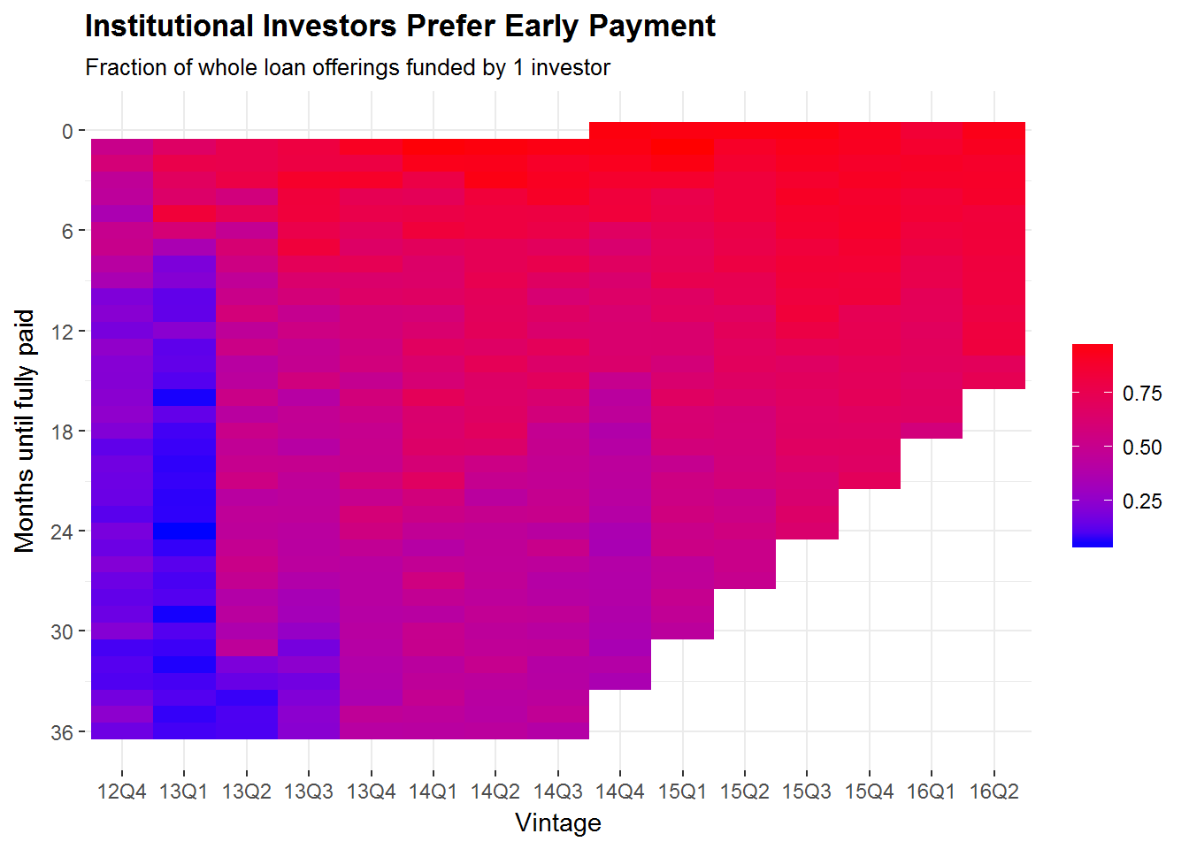

There are at least two explanations that are consistent with the above observations.

First is Lending Club’s policy governing servicing fees:⁵

Note investors generally pay us a servicing fee equal to 1% of payment amounts received from the borrower. Whole loan purchasers pay a monthly servicing fee of up to 1.3% per annum on the month-end principal balance of loans serviced.

When fees are a proportion of remaining principal, investors will prefer early payment—even if it means accepting higher default risk, as suggested by the first plot.⁶ (See this supplemental post for a mathematical explanation.) Thus servicing fees may act as a mechanism to influence portfolio selection for each of the two types of investors.

A second possible explanation concerns the availability of liquidity. On Lending Club, loans are 3-year and 5-year fixed income investments, and it may take that long to realize the full return from the initial capital. Retail investors have access to a Note Trading Platform via Folio Investing, which acts as a secondary market to provide liquidity. Institutional investors have no analogous avenues to trade whole loans, which means the only liquidity option is to fund loans whose borrowers will prepay. Like servicing fees, this can also be viewed as a structural feature of the market that might produce the observed patterns.

Conclusion

As large institutional investors have eclipsed⁷ small-money retail investors on Lending Club and other platforms, it has become increasingly important to understand how these two types interact through their investment choices. In one simplified view, they compete for high-quality loans that will yield the most attractive returns, prompting questions related to the fairness of marketplace design. This is an especially salient issue for Lending Club since whole loan investors are given priority in loan selection.

This post presented evidence that institutional and retail investors have different preferences over loan portfolios, and that these differences may be induced by features of Lending Club’s market design, namely servicing fees and access to liquidity. While the analysis is far from complete, it blunts the appeal of the pure competitive view, instead suggesting that platforms can deliver fair opportunities for attractive returns to both types of investors.